Notes on hyperbolic space (and embedding trees in it)
13 Jul 2020
#
Note: this is simply a compilation of blocks of texts and images gathered from around the internet that I found informative and useful. The sources are listed at the bottom but not directly in text. Apologies and thanks to the authors. Thanks to Maria who helped clarify some things.
1. Euclid’s postulates (The Elements, 300 BC, written in Alexandria)
Grade school mathematics is taught using Euclidean geometry. This assumes Euclid’s axioms, which he intended to be the basis of all geometry.
- A straight line segment can be drawn joining any two points.
- Any straight line segment can be extended indefinitely in a straight line.
- Given any straight lines segment, a circle can be drawn having the segment as radius and one endpoint as center.
- All rights angles are equal to each other
However, one of them was a great source of debate between mathematicians.
The “Parallel Postulate”
- If two lines are drawn which intersect a third in such a way that the sum of the inner angles on one side is less than two Right Angles, then the two lines inevitably must intersect each other on that side if extended far enough. This postulate is equivalent to what is known as the Parallel Postulate.
This has been more recently rephrased as Playfair’s axiom: **
In a plane, given a line and a point not on it, at most one line parallel to the given line can be drawn through the point.
Many geometers made attempts to prove the parallel postulate. Some tried to prove it by assuming its negation and trying to derive a contradiction. Foremost among these were Proclus, Ibn al-Haytham, Omar Khayyám, Nasīr al-Dīn al-Tūsī, Witelo, Gersonides, Alfonso, and later Giovanni Gerolamo Saccheri, John Wallis, Johann Heinrich Lambert, and Legendre. Their attempts were doomed to failure — the Parallel Postulate need not hold true in all cases — but their efforts led to the discovery of hyperbolic geometry.
2. Non Euclidian geometries
Although it at first seems unnatural to think about parallel lines performing in “new” ways, hyperbolic surfaces can be found in nature. Two common examples are sea slugs (Figure 1) and lettuce (Figure 2). The wavy structure is the tip-off that their surfaces exhibit hyperbolic geometry. This is because, while a Euclidean surface has curvature equal to zero everywhere, a hyperbolic surface has constant negative curvature (for comparison, a sphere has constant positive curvature).
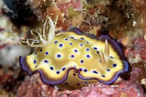

Figure 1 - a sea slug and Figure 2 - lettuce
**
There are many different kinds of curvature, and they can be with respect to either curves or surfaces (hypersurfaces) with the latter having many different variants. The basic idea behind all these different definitions is that curvature is some measure by which a geometric object deviates from a flat plane, or in the case of a curve, deviates from a straight line.
Gaussian Curvature
Gaussian curvature is a measure of curvature for surfaces (2D manifolds). Let’s take a look at Figure 3 which shows the three different types of Gaussian curvature and Figure 4 showing how a triangle behaves differently on differently curved surfaces.
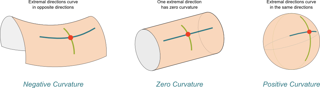
Figure 3: Examples of the three different types of Gaussian curvature (source: Science4All).
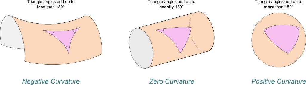
Figure 4: Deviation of a triangle under the three different types of Gaussian Curvature (source: Science4All).
3. Hyperbolic geometry and the Poincaré disc model
In hyperbolic geometry Euclid’s 5th becomes:
For any given line R and point P not on R, in the plane containing both line R and point P there are at least two distinct lines through P that do not intersect R.
Hyperbolic geometry has many interesting properties that counter our ingrained Euclidean intuition. To understand them, we will explore an important model of hyperbolic space: the Poincaré disc model.
We can imagine hyperbolic space as an open disk in the complex plane \(C\). We think of the space in the disk getting infinitely more “dense” as we approach the boundary of the disc, so the distance of a straight line between two points get longer as we approach the boundary. Thus, the shortest path between two points may be curved to take advantage of the “less dense” area towards the center of the disc.
In the Poincaré disk, all points are in the interior of the unit disk in two dimensions. Hyperbolic space is a beautiful and sometimes weird place. The “shortest paths”, called geodesics, are curved in hyperbolic space. It turns out that the shortest distance between two points lies along the arc of a circle that is perpendicular to the boundary.
In Figure 6 the geodesic between A and B is the arc length of the given circle.
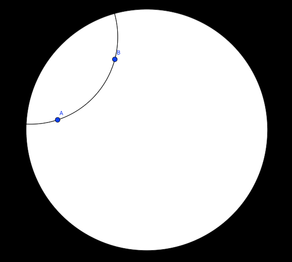
Figure 5: A geodesic between points A and B
The figure below shows parallel lines (geodesics); for example, there are infinitely many lines through a point parallel to a given line.
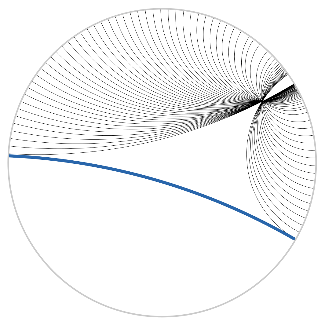
Figure 6: from wikipedia
The biggest thing to realize is, first, there are an infinite number of points within the circle – infinities are hard to reason about. Second, we need to throw away our Euclidean sensibilities and intuition. For example, we’ll see below that the “distance” between points grows exponentially as we move towards the outside of the Poincaré disk. We need to use a combination of the math and throwing away our old intuition in order to understand these non-flat models of geometry.
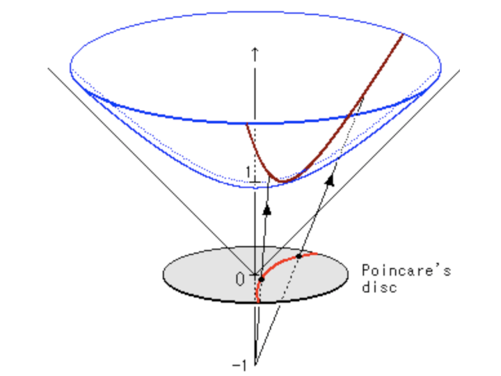
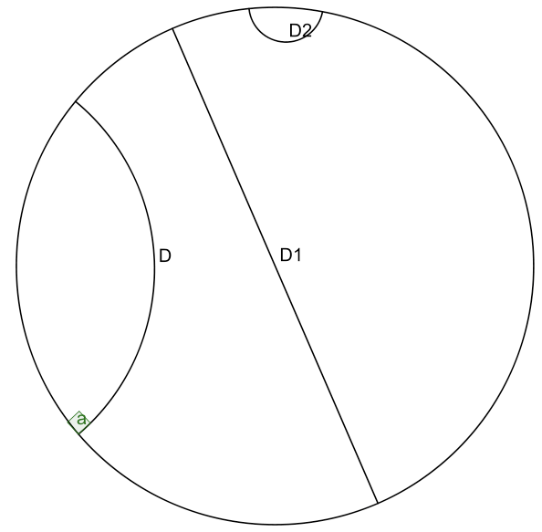
Figure 7 & 8
A few notable points:
- The arcs never reach the circumference of the circle. This is analogous to the geodesic on the hyperboloid extending out the infinity, that is, as the arc approaches the circumference it’s approaching the “infinity” of the plane.
- This means distances at the edge of the circle grow exponentially as you move toward the edge of the circle (compared to their Euclidean distances).
- Each arc approaches the circumference at a 90 degree angle, this just works out as a result of the math of the hyperboloid and the projection. The straight line in this case is a point that passes through the “bottom” of the hyperboloid $(0,0,1)$.
- Lines that are parallel can actually diverge from each other (also known as “ultra parallel”). This is a consequence of changing Euclid’s 5th postulate regarding parallel lines. A more clear example is Figure 6. Here we see that we can have an infinite number of lines (black) intersecting at a single point and still be parallel to another line (blue).
4. Tesselation of the hyperbolic plane (an Escher interlude)
Anyone who has looked at a tiled bathroom floor is familiar with the idea of tessellations: If we repeat a pattern of polygons, we can create a pattern over a large space. Someone who has attempted to tile their own bathroom floor may have noticed that not all tile shapes fit together nicely in a pattern. Note that a bathroom floor is an example of a Euclidean space, a geometry in which it turns out to be relatively difficult to happen upon a true tessellation. In contrast, hyperbolic space is relatively easy to tessellate.
M. C. Escher (1898-1972) is known for his mind-boggling artwork that challenges our sense of space. Although many of his works are artistic renditions of deep mathematical ideas, he had no formal training in mathematics. Escher’s art branched into tessellations of the plane. He was inspired by the idea of “approaches to infinity” and began by playing with flat surfaces and spheres.
Escher’s ideas about structure, pattern, and infinity were suddenly enhanced when he came across the work of geometer H. S. M. Coxeter (1907-2003). Coxeter and Escher struck up a correspondence when Coxeter hoped to use Escher’s unique depictions of symmetry in a presentation for the Royal Society of Canada. Coxeter sent Escher a copy of the talk, which included an illustration depicting a tessellation of the hyperbolic plane (Figure 9).
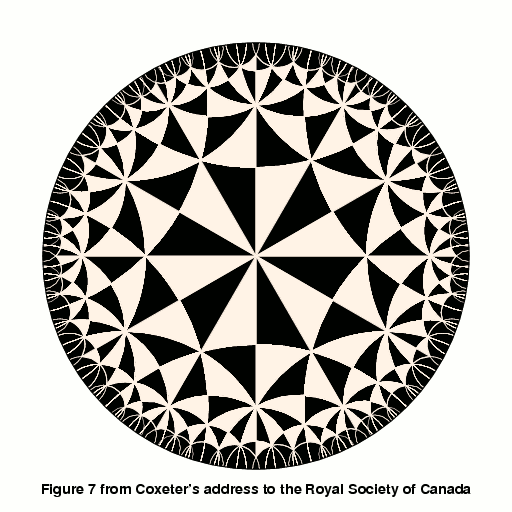
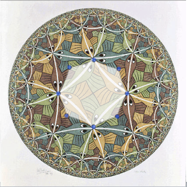 Figure 9: Coxeter’s tessellation.
Figure 10: “For me it remains an open question whether [this work] pertains to the realm of mathematics or to that of art.” -M. C. Escher
Escher created five works inspired by hyperbolic plane tessellations: Circle Limits I-IV and Snakes. His goal with creating these was to depict infinity in a finite space. When thinking about the increased “density” as we approach the edge, it should not be surprising that polygons appear smaller as we approach the boundary. Despite this, the areas stay constant (recall that it depends only on the angles!).
5. The Limitations of Euclidean Space for Hierarchical Data
The whole reason why we went through that primer on hyperbolic geometry is that we want to embed data in it! Consider some hierarchical data, such as a tree. A tree with branching factor 𝑏 has \((𝑏+1)𝑏^{𝑙−1}\) nodes at level 𝑙 and \(\frac{(b+1) b^{l}-2}{b-1}\) nodes on levels less than or equal to 𝑙. So as we grow the levels of the tree, the number of nodes grows exponentially.
There are really two important pieces of information in a tree. One is the hierarchical nature of the tree: the parent-child relationships. The other is a relative “distance” between the nodes. Children and their parents should be close, but leaf nodes in totally different branches of the tree should be very far apart (probably somehow proportional to the number of links).
Let’s imagine putting this into a Euclidean (say 2D) space. First, we would probably put the root at the origin. Then, place the first level equidistant around it. Then place the second level equidistant from all those points. Figure 11 shows these two levels.

Figure 11.
You can see we’re already running out of space. The hierarchical links are sort of represented (distances between child/parent are maintained), but importantly, the distances between siblings gets smaller. Look at the leaf nodes which are squeezed at the edge because we don’t have enough “space”. One way around, might be to increase dimensions but then you’d need to increase those with the number of levels you have, which brings a whole host of other problems. Long story short, Euclidean space isn’t a good representation for graph-like data.
6. Embedding trees in hyperbolic space
It shouldn’t be a surprise at this point to know that hyperbolic space is a good representation of hierarchical data. Using the same sort of algorithm as we tried above of placing the root at the center and spacing the children out equidistant recursively does work in hyperbolic space. The reason is that distances grow exponentially as we move toward the edge of the disk, eliminating the “crowding” effect we saw above. Figure 12 shows a visualization for a tree with branching factor two.
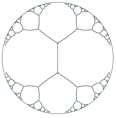
Figure 12.
Of course, Figure 12 looks crowded at the lower levels just like the previous figure but that’s only because hyperbolic space is hard to visualize intuitively. In fact all the points in Figure 12 are equidistant from their parent, and siblings and cousins nodes are much further apart then they appear. So crowding in fact isn’t much of an issue.
The hyperbolic distance between two points x and y has a particularly nice form:
\[d_{p}(\boldsymbol{x}, \boldsymbol{y})=\operatorname{arcosh}\left(1+2 \frac{\|\boldsymbol{x}-\boldsymbol{y}\|^{2}}{\left(1-\|\boldsymbol{x}\|^{2}\right)\left(1-\|\boldsymbol{y}\|^{2}\right)}\right)\]Consider the distance from the origin \(d_{H}(O, x)\). Notice as \(x\) approaches the edge of the disk, the distance grows toward infinity, and the space is increasingly densely packed. Let’s dig one level deeper to see how we can embed short paths that define graph-like structures—in a much better way than we could in Euclidean space.
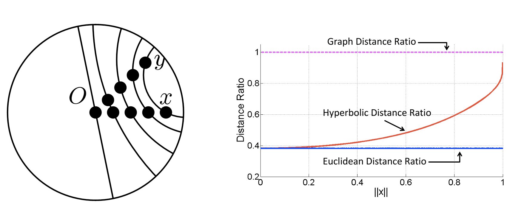
Figure 13: \(\Vert{x}\Vert\) on the right figure (x-axis) represents the distance of \(x\) and \(y\) to \(O\).
The goal when embedding a graph \(G\) into a space \(V\) is to preserve the graph distance (the shortest path between a pair of vertices) in the space \(V\).
If \(x\) and \(y\) are two vertices and their graph distance is \(d(x,y)\), we would like the embedding to have \(d_{V}(x,y)\) close to \(d(x,y)\).
Now consider two children \(x, y\) of parent \(z\) in a tree. We place \(z\) at the origin \(O\). The graph distance is \(d(x,y)=d(x,O)+d(O,y)\), so normalizing we get: \(\frac{d(x, y)}{d(x, O)+d(O, y)}\).
Time to embed \(x\) and \(y\) in two-dimensional space. We start with \(x\) and \(y\) at the origin, and with equal speed move them toward the edge of the unit disk away from the origin \(O\) (see Figure 13, left) represented by the norm of \(x\) (\(\Vert{x}\Vert\)). What happens to their normalized distance?
In Euclidean space, \(\frac{d_{E}(x, y)}{d_{E}(x, O)+d_{E}(O, y)}\) is a constant, so Euclidean distance does not seem to capture the graph-like structure.
In hyperbolic space, \(\frac{d_{H}(x, y)}{d_{H}(x, O)+d_{H}(O, y)}\) (red line), when \(x\) and \(y\) are close to \(O\) (\(\Vert{x}\Vert \approx 0\)), their relative hyperbolic distance looks more like their Euclidean distance. As the distance gets larger, hyperbolic distance begins to look more like the graph distance and approaches 1.
We can’t exactly achieve the graph distance in hyperbolic space, but we can get arbitrarily close! The trade off is that we have to make the edges increasingly long, which pushes the points out the edge of the disk.
Sources:
Tessellations of the Hyperbolic Plane and M.C. Escher - Allyson Redhunt
Hyperbolic geometry - Wikipedia